Intro to multi-armed bandit, some coding and math
Imagine yourself in a casino and you’re trying to get some money. There are thousands of slot machines. Each one of them has a lever, that if you pull it, you might receive nothing or some money. So, can you tell me some strategy to maximize your profits?
This is a classical reinforcement learning problem called multi-armed bandit. You have choices among thousands of slot machines, each action selection is like choosing a bandit and pulling its lever, then you receive a numerical reward from an unknown distribution. Your main goal is to maximize the expected total reward over some time steps.[1]
Sample-averaging method
In order to tackle this problem, let’s work just with one-armed bandit. Let’s say each slot machine has an expected reward, so let’s call it action-value. This value can be naively calculated by taking the average of all the rewards of that specific slot machine.
That’s given by:
By the law of the large numbers, as , this estimate approaches the expected distribution.
Now, let’s check it out this method…
np.random.seed(42)   # for reproducibility
bandit = Bandit(1/3) # assuming a stationary distribution

time_steps = [100, 500, 1000, 5000, 10000, 1000000]

for time_step in time_steps:
    rewards = []
    for _ in range(time_step):
        r = bandit.pull()
        rewards.append(r)

    expected_reward = np.mean(rewards)
    print(f'Timesteps: {time_step:9} - Q(a): {expected_reward:.4f} | MAE: {np.abs(expected_reward - bandit.p):.4f}')
Output
Timesteps:       100 - Q(a): 0.4100 | MAE: 0.0600
Timesteps:       500 - Q(a): 0.3380 | MAE: 0.0120
Timesteps:      1000 - Q(a): 0.3580 | MAE: 0.0080
Timesteps:      5000 - Q(a): 0.3536 | MAE: 0.0036
Timesteps:     10000 - Q(a): 0.3537 | MAE: 0.0037
Timesteps:   1000000 - Q(a): 0.3496 | MAE: 0.0004
Here we can see that as the number of steps increase, the expected reward approaches the real distribution.
Although it’s a simple implementation, this code doesn’t perform very well. This is due to the fact that we’re recording all the rewards. Consequently, the memory and computational tasks will grow over the time.
Incremental implementation
So, how can we improve the algorithm? One way is to rearrange the formula’s terms and turn it incremental.
Let’s say is the estimate for the reward.
And since , we can substitute the summatory term, then…
We can express this as:
This expression is like gradient descent where we take small steps toward the target.
Let’s check it out…
bandit = Bandit(1/3) # assuming a stationary distribution

time_step = 10000

Q = .0
k = 1
for _ in range(time_step):
    r = bandit.pull()

    Q = Q + 1./k * (r - Q)
    k += 1

print(f'Timesteps: {time_step:9} - Q(a): {Q:.4f} | MAE: {np.abs(Q - bandit.p):.4f}')
Output
Timesteps: 10000 - Q(a): 0.3356 | MAE: 0.0023
An awesome approach! The computational task is small and we store just and (the current expected reward).
Exploration and Exploitation Dilemma
All right, now let’s return to our original problem, there are thousand of slot machine, how can we maximize our profits over the time?
Since we can estimate the expected reward of each slot machine, it will exist one that will have the highest action-value. Those are called greedy-actions.
Greedy-actions are defined as:
Since we don’t have any knowledge about the slot machines, we have to explore them in order to improve our estimates. And then, we can exploit our knowledge in order to optimize our expected total reward.
In a short run, the rewards might be lower while exploring, however in a long run the return might be higher.
So, when should we explore and when should we exploit?
There is a near greedy approach called -greedy method. With a probability of , we’ll be choosing the greedy action, otherwise we’ll be acting randomly.
Let’s see how -greedy method works…
# assuming a stationary distribution
probs = [.01, .20, .30, .50, .65, .70]
bandits = Bandits(probs)

time_step = 10000

epsilon = 1.
rewards = []
Q = np.zeros(bandits.n)
k = np.ones_like(Q)
for _ in range(time_step):

    if np.random.random() < epsilon:
        action = np.random.choice(range(bandits.n)) # exploration
    else:
        action = np.random.choice(np.argwhere(Q==np.amax(Q)).ravel()) # exploitation
    r = bandits.pull(action)

    Q[action] = Q[action] + 1./k[action] * (r - Q[action])
    k[action] += 1
    rewards.append(r)

    epsilon = max(epsilon-.0001, .01)
Here, we assigned . This is to force the exploration phase. However, as the time pass by, we slightly decrement it. Then, it will be exploring more over the time.
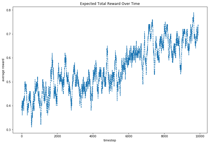
Here we can see our expected total reward over the time. We can see that it’s low in the exploration phase, however it increases while exploiting the acquired knowledge.
Summary
Here we introduced the multi-armed bandit problem. This is somehow a simplification of the reinforcement learning. Multi-armed bandit is a nonassociative problem, that is, the problem doesn’t have states which could influence in our decision making. However, we could extend this idea to an associative problem. For example, if each slot machine has a colored light that changes over the time.
We tackled the problem solving the one-armed bandit through sample-averaging and incremental approach, and finally we solved the multi-armed bandit using the -greedy method to explore and exploit our options.
So, that’ all! Hope you enjoyed and I drop a notebook with the implementation below.
References
- Reinforcement Learning: An introduction, Sutton and Barto
- Multi-armed bandit (jupyter notebook)