Checking independence between categorical variables

Whenever you’re exploring your dataset, you may want to check the correlation between some variables.
However, if the variables are categorical, how can we check relationship between them?

The chi-squared distribution

In order to make inference between our variables, we need to use the chi-squared distribution $(\chi^2)$ .

The chi-squared distribution is a family of distributions and it can be achieved by summing the square of $k$ independent normally distributed random variables.

A random variable normally distributed is given by:

$X \sim N(0, 1)$

In other words:

The expected value is equal to ZERO
$E[X] = 0$
The variance is equal to ONE
$Var[X] = 1$

By squaring the random variable, we’ll get a new random variable.

$\chi^2_1 = X^2$

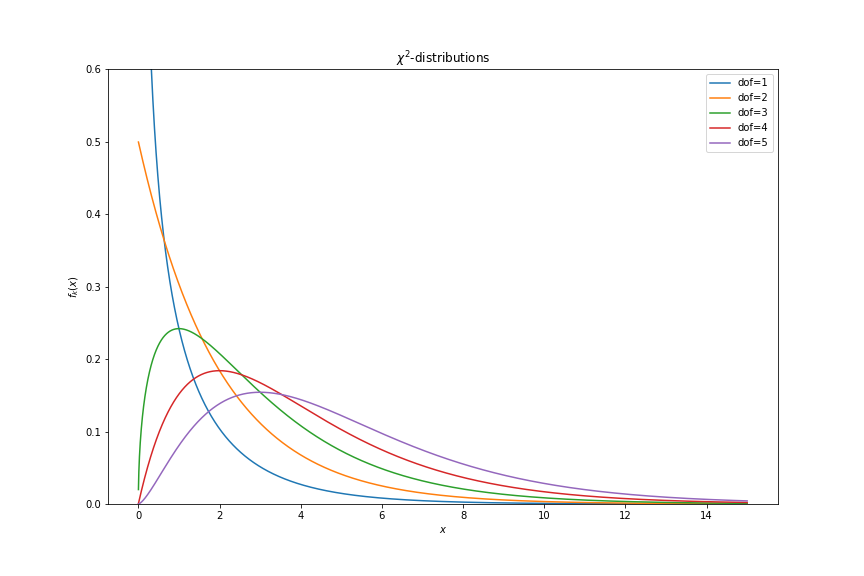
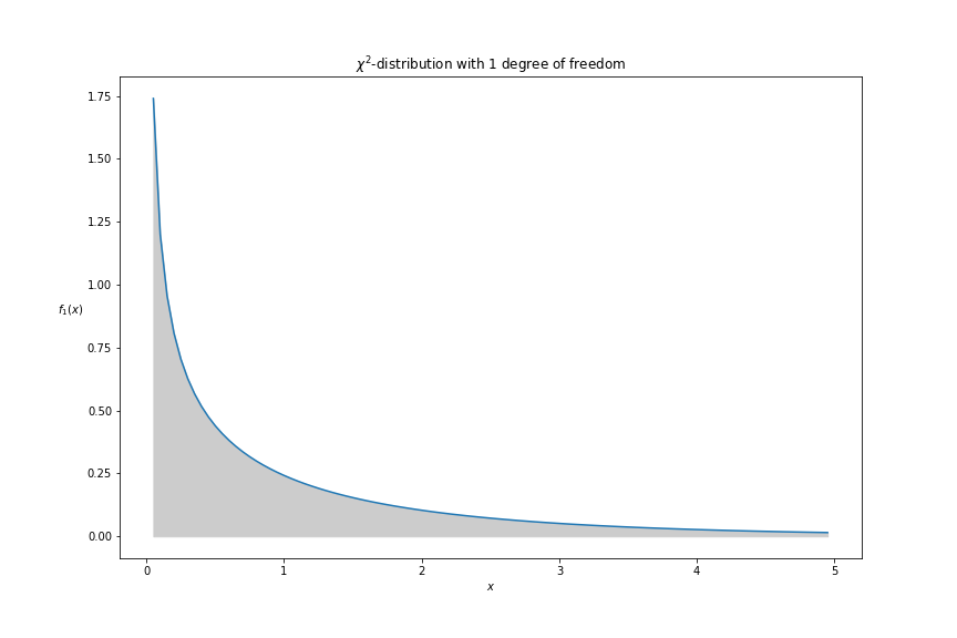
This random variable is a chi-squared distribution with 1 degree of freedom.

Now, if we square 2 normally distributed random variables and sum them, we’ll get another chi-distribution with 2 degrees of freedom.

$\chi^2_2 = X^2 + X^2$

The distributions will have the following shapes…

So, how it works?
Let’s say you sampled 3 values from a normal distribution, what is the probability that the sum of the squares is greater than 8?

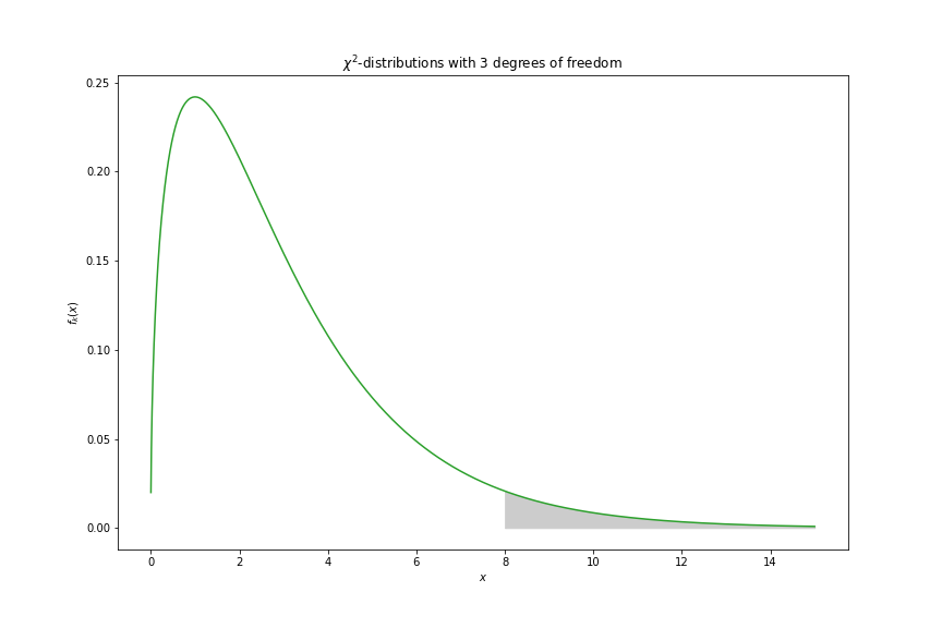
By looking in the previous image, we can see that we want the shaded area of the distribution.
If we look at the chi-square table with 3 degrees of freedom, we can see that values greater than 8 are likely to happen with a probability lower than 5%.

Since these distributions are well known, we can test how well theoretical distributions explain observed ones.

Demonstration

For demonstration, we’ll be using Kaggle’s titanic dataset.

Here, our main goal is to check if:

the survivability has any significant relationship with passenger’s gender.

So, lets import our dataset.

np.random.seed(42)        # for reproducibility
DIR = 'datasets/titanic/' # dataset directory

data = pd.read_csv(f'{DIR}/train.csv', usecols=['Survived', 'Sex'])
data.head()

The output should be something like this…

Survived	Sex
0	male
1	female
1	female
1	female
0	male

Checking relationship

In order to do the hypothesis test, we’ll need to get the contingency table.
We can achieve this by using pandas.crosstab function.

X = data.sample(90)
crosstab = pd.crosstab(X['Survived'], X['Sex'])

print(crosstab)

The contingency table should be something like this…

Sex	female	male
Survived
0	9	45
1	28	8

Now, we’ll need to calculate the degrees of freedom (dof).
The dof is defined as $(columns - 1) \times (rows - 1)$ .

def get_dof(crosstab):
    cols = len(crosstab.columns)
    rows = len(crosstab.index)

    return (cols-1) * (rows-1)

dof = get_dof(crosstab_by_sex)
print(f'Degrees of freedom is: {dof}')

Output: Degrees of freedom is: 1

So, we’ll need to calculate the chi-squared statistic.
Chi-squared statistic is defined as…

$\chi^2 = \sum_i \frac{(o_i - e_i)^2}{e_i}$

where:

$o_i$ - it’s the i^th observed value;
$e_i$ - it’s the i^th expected value;

We already have the observed values, so we need to calculate the expected values.

def get_expected_value(crosstab):
    total = np.sum(crosstab)
    
    total_by_rows = np.sum(crosstab, axis=0, keepdims=True)
    total_by_cols = np.sum(crosstab, axis=1, keepdims=True)
    
    return total_by_rows*total_by_cols/total

expected = get_expected_value(crosstab.values)
print(expected)

Output:
[[23.4 36.6]
[15.6 24.4]]

Now, we just need to calculate the chi-square statistics.

def calc_chi2_stat(observed, expected):
    return np.sum((observed-expected) ** 2 / expected)

chi2_stat = calc_chi2_stat(crosstab.values, expected)
print(f'chi-square statistic is {chi2_stat:.2f}')

Output: chi-square statistic is 31.45

With chi-square statistic in hand, we just need to calculate the p-value.

The intution here is that the shaded area is equal to 1.
So, if we calculate the cdf until the chi2-stat, the p_value is the complement of this probability, then we can use it to make our inference.

def calc_p_value(chi2_stat, dof):
    return 1. - stats.chi2.cdf(chi2_stat, df=dof)

p_value = calc_p_value(chi2_stat, dof)

So, we’ll be using alpha equals to 5% and our hypothesis test is…
$H_0$ : Both variables are independent - i.e. - they don’t have any association.
$H_A$ : Both variable are dependent - i.e. - they’re associated.

If our p_value is lower than our alpha, we can reject the null hypothesis ( $H_0$ ) and conclude that the alternative hypothesis is true.

alpha = .05
if p_value < alpha:
    print('Reject null hypothesis: Both variables are dependent')
else:
    print('Failed to reject null hypothesis: Both variables are independent')

Output: Reject null hypothesis: Both variables are dependent

Finally, as we can see, both variables are dependent and actually we can notice this relationship just by looking in the following plot.

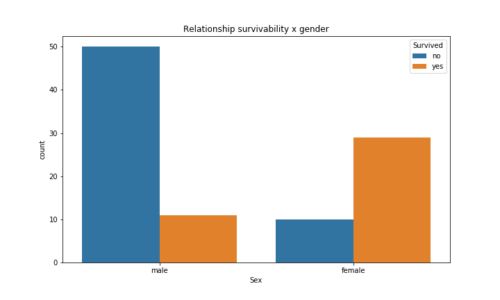
So, why we had to do all of this stuff if we could notice just by this simple plot?

Well, interpreting the barplot might be somehow subjective, that is, it will depends on who is analysing.
However, with this hypothesis testing, we could conclude if the variables have significant relationship and moreover, sometimes it will be hard to see the relationship in a plot, so it will be more straightforward if we just do the independence test.

The chi-squared distribution

Demonstration

Checking relationship

References